Introduction
Analytical method development has evolved far beyond the traditional “trial-and-error” approach. In the modern regulatory landscape, analytical laboratories are expected to apply the same scientific rigor used in product development to the design of their analytical methods. The introduction of ICH Q14 (Analytical Procedure Development) and the revised ICH Q2(R2) guidelines has officially established the Quality-by-Design (QbD) framework as a regulatory expectation, not merely a scientific preference.
In practice, this means that an analytical method is no longer judged solely by its validation results it must demonstrate a scientific understanding of how each variable influences method performance, reliability, and control. This shift marks the beginning of the analytical lifecycle management era, where methods are developed, verified, and maintained within a defined design space supported by continuous improvement.
For regulatory specialists and analytical scientists alike, this change introduces both challenges and opportunities. A method designed using QbD principles can offer:
- Enhanced robustness against small variations in parameters.
- Greater regulatory flexibility (e.g., minor post-approval changes within the MODR require no revalidation).
- A documented, traceable risk-based justification for each analytical choice.
To help laboratories integrate these principles effectively, this article provides a step-by-step, actionable roadmap that bridges conventional method development with QbD-driven analytical design. Each step focuses on practical actions, supported by real laboratory examples, risk management tools, and regulatory references from ICH Q14, Q9(R1), USP <1220>, and FDA/EMA guidance.
The framework begins by defining the Analytical Target Profile (ATP),the foundation of all subsequent decisions and progresses through identifying critical parameters, performing risk assessment, applying Design of Experiments (DoE), and establishing the Method Operable Design Region (MODR). It concludes with lifecycle control and continuous performance monitoring, ensuring compliance with the newest regulatory expectations.
This structured roadmap empowers analytical teams to move from empirical development to science-based, risk-managed, and regulatory-aligned method design setting a new benchmark for analytical excellence in pharmaceutical research and quality control.
Step 1: Define the Analytical Purpose and Establish the Analytical Target Profile (ATP)
Objective:
To clearly identify what the analytical method is intended to measure and how its performance will be evaluated, forming the foundation for all subsequent development and validation steps.
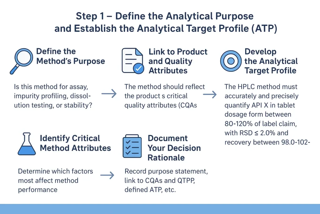
1.1. Define the Method’s Purpose:
Every analytical method must begin with a well-defined intended use. Ask:
- Is this method for assay (quantifying the main component)?
- For impurity profiling?
- For dissolution testing?
- Or for stability-indicating purposes?
The method’s goal determines its sensitivity, selectivity, and robustness requirements.
1.2. Link to Product and Quality Attribute
The analytical method must directly reflect the product’s Critical Quality Attributes (CQAs).
For instance:
- Purity method: linked to CQA of related substances.
- Dissolution method: linked to CQA of drug release rate.
- Assay method: linked to CQA of dosage accuracy.
These CQAs originate from the Quality Target Product Profile (QTPP) — a key concept in ICH Q8 (R2) and ICH Q6A.
Tip
Always align the analytical target (ATP) with the intended control strategy in the overall pharmaceutical development plan.
1.3. Develop the Analytical Target Profile (ATP)
The ATP acts as a “performance contract” for the method.
It defines:
- What the method measures
- How well it must perform
- Under what conditions it should be reliable
1.4. Identify Critical Method Attributes (CMAs)
From the ATP, determine which factors most affect method performance, e.g.:
- Column type (C18, phenyl, etc.)
- Mobile phase pH
- Detector wavelength
- Flow rate
- Temperature
These become your Critical Method Parameters (CMPs), to be optimized later in Step 3.
1.5. Document Your Decision Rationale
In your development record, include:
- Purpose statement
- Link to CQAs and QTPP
- Defined ATP
- Preliminary risk assessment identifying CMAs and CMPs
Reference template for documentation:
| Section | Description |
|---|---|
| Method Type | (e.g., HPLC assay, Dissolution test) |
| Analyte | Active ingredient name |
| Matrix | Dosage form or sample medium |
| Intended Use | QC release / Stability / Development |
| Performance Criteria | Accuracy, precision, linearity ranges |
| Regulatory Reference | ICH Q8(R2), ICH Q2(R2), USP <1225> |
- ICH Q8 (R2): Pharmaceutical Development
- ICH Q2 (R2): Validation of Analytical Procedures
- USP <1225>Validation of Compendial Procedures
Step 2: Identify Critical Method Attributes (CMAs) and Critical Method Parameters (CMPs)
Objective:
determine which method outputs (CMAs) must be controlled to meet the ATP and which operational variables (CMPs) influence those outputs, so you can focus risk assessment and experimentation where it matters.
Step 2.1: Define the terms
- CMA (Critical Method Attribute): a measurable outcome of the method that directly affects decision-making (e.g., resolution between API and impurity, peak symmetry, %RSD of assay, limit of quantitation).
- CMP (Critical Method Parameter): an operational factor that can change a CMA (e.g., mobile-phase pH, flow rate, column chemistry, detector wavelength).
Step 2.2: Map ATP → CMAs
Consider Practical Factors
- Take the ATP from Step 1 and list the performance requirements (accuracy range, precision limit, detection limit, throughput).
- For each ATP requirement, assign the CMAs that directly demonstrate it.
- Example: ATP = “Assay accuracy 98–102%” → CMAs = recovery (%) and %RSD (repeatability).
- Matrix Effects: Assess interference from buffers, excipients, or solvents.
Step 2.3: Brainstorm CMPs with an Ishikawa
- Convene a short cross-functional session (analyst + instrument tech + QA).
- Use an Ishikawa (fishbone) diagram and populate categories: Instrument, Reagents/Materials, Method Conditions, Analyst, Environment.
- For each CMA, list potential CMPs.
Step 2.4: Prioritize CMPs
- For each CMP estimate: Severity (impact on CMA), Likelihood (how often it varies), and Detectability (how easy to monitor).
- Flag high-priority CMPs that score high for severity and likelihood — these become inputs to the FMEA in Step 3 and to your DoE plan in Step 4.
Step 2.5: Create a CMA–CMP relationship table
| CMA | Key CMP | Why Critical | Immediate control suggesstion |
|---|---|---|---|
| Resolution (API/imp) | pH, % organic, column type | Affects selectivity → false negative/positive | Include pH in DoE; set SOP for mobile-phase prep |
| %RSD (assay) | Injection volume, sample prep | Poor precision invalidates results | Autosampler maintenance; analyst training |
Quick tips
- Use prior method data for similar molecules to shorten the CMP list.
- Document rationale for each CMP — regulators expect traceable scientific reasoning.
- Keep the list focused: it’s better to fully evaluate 3–5 CMPs than superficially list 20.
Step 3: Perform Risk Assessment (FMEA or Risk Matrix)
Objective
Prioritize which method parameters (CMPs) pose the greatest risk to the critical method attributes (CMAs), ensuring that experimental work focuses on what truly affects method performance and regulatory reliability.
Step 3.1: Define your risk assessment approach
Two common tools are acceptable per ICH Q9(R1) and ICH Q14 Annex 1:
- FMEA (Failure Mode and Effects Analysis) — quantitative, assigns scores for each risk.
- Risk Matrix — qualitative, uses “Low/Medium/High” ranking.
Step 3.2: Prepare your input data
Gather from Step 2:
Example inputs:
- CMP: pH of mobile phase → CMA: Resolution
- CMP: Flow rate → CMA: Tailing factor
- CMP: Column temperature → CMA: Retention time
Step 3.3: Apply the FMEA scoring system
Each CMP–CMA pair is evaluated for:
- Severity (S): How serious is the effect if the parameter drifts? (1–10)
- Occurrence (O): How likely is it to vary? (1–10)
- Detectability (D): How easy is it to detect before impact? (1–10)
Calculate: RPN (Risk Priority Number) =S×O×D
CMP CMA S O D RPN Interpretation Mobile phase pH Resolution 9 6 3 162 high risk Flow Rate Tailing 7 5 4 140 moderate Column Temperature Retention time 5 3 2 30 low
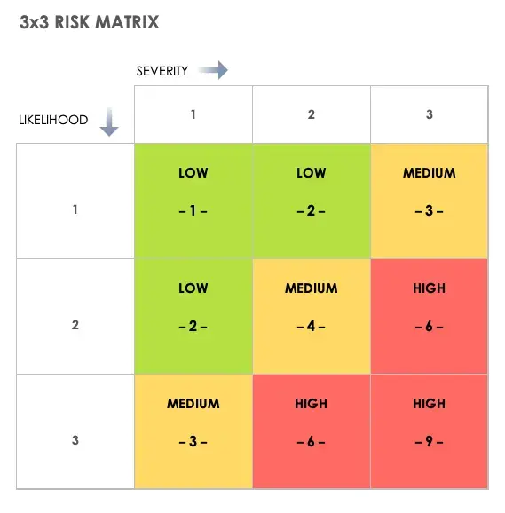
Step 3.4: Visualize with a risk matrix
If qualitative, create a 3×3 grid: Severity (Low–High) × Likelihood (Low–High).
Plot each CMP to highlight high-risk zones visually.
Tip
Use color-coding (red = high, yellow = moderate, green = low) for clear communication in reports or regulatory dossiers.
Step 4: Conduct Design of Experiments (DoE)
Design of Experiments (DoE) is the structured, statistical approach that reveals how Critical Method Parameters (CMPs) influence Critical Method Attributes (CMAs). In analytical Quality-by-Design (QbD), DoE is the bridge between theory and experimental confirmation, it converts the risk assessment into scientifically defensible data.
4.1 Define the Objective
Before any experiment, clearly state the purpose:
- Are you screening to identify significant parameters?
- Are you optimizing to find the ideal combination of variables?
- Or are you confirming the robustness of an established region?
4.2 Select the Experimental Design Type
Match your DoE type to the study goal:
- Screening designs (e.g., Plackett–Burman, 2ⁿ factorial) → identify main factors.
- Optimization designs (e.g., Central Composite, Box–Behnken) → explore curvature and interactions.
- Robustness designs → evaluate stability around the target condition.
Actionable Tip
Begin with a 2³ full factorial to study three parameters at two levels (low/high). Expand to response surface designs if interactions are significant.
4.3 Define Variables and Ranges
Base each range on prior knowledge, literature, or system suitability data
| Parameter | Low level | High Level | Justification |
|---|---|---|---|
| pH | 6 | 7 | Within buffer capacity range |
| Flow Rate | 0.9 mg/ml | 1.1 mg/ml | Typical range for column stability |
| % Organic | 55 | 65 | Affects retention and resolution |
4.4 Execute the Experimental Runs
Perform runs in randomized order to minimize systematic bias.
Maintain consistent instrument conditions (column, temperature, injection volume).
After each run, document key CMAs—retention time, resolution, peak symmetry, % RSD.
Practical Tip
Automate runs through a validated sequence table; this minimizes analyst-induced variability.
4.5 Analyze the Data
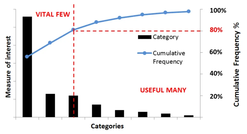
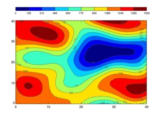
Use statistical software (e.g., Design-Expert®, Minitab®, JMP®):
- Generate Pareto charts for factor significance.
- Construct main effects and interaction plots.
- Evaluate response surface models and ANOVA p-values (< 0.05) for significance.
4.6 Confirm Optimal Conditions
Use model predictions to identify an operating region that achieves target CMAs.
Verify with confirmation runs at predicted optimum points.
4.7 Key Reference
- FDA (2015) Analytical Procedures and Methods Validation Guidance
- ICH Q14 §4.2 — “Multivariate Experiments for Analytical Method Understanding”
Step 5: Establish the Method Operable Design Region (MODR)
Once the Design of Experiments (DoE) confirms how your Critical Method Parameters (CMPs) affect Critical Method Attributes (CMAs), the next task is to translate these statistical relationships into a Method Operable Design Region (MODR)—the scientifically justified zone where your method consistently meets its Analytical Target Profile (ATP).
MODR represents the “proven acceptable range” (PAR) for each critical parameter and their interactions. It’s the practical expression of method robustness, giving both scientists and regulators a data-driven assurance of performance consistency.
5.1 Define the Boundaries of the MODR
Using DoE results, identify the parameter ranges where all critical attributes meet predefined acceptance criteria.
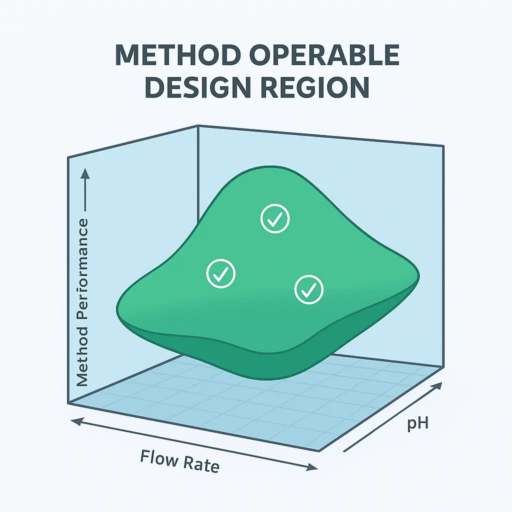
Example: For an HPLC assay of Drug X:
- pH: 6.4–6.8
- Flow rate: 0.95–1.05 mL/min
- Organic phase: 58–62% acetonitrile
Within this region, the method maintains:
- Resolution ≥ 2.0
- Tailing ≤ 1.5
- %RSD ≤ 2.0
Actionable Tip
Avoid setting arbitrary wide ranges. Instead, use model predictions and confirmatory runs to ensure compliance within boundaries.
5.2 Establish Design Space Interaction Map
Visualize how multiple factors interact to affect the response.
- Contour plots and response surface plots help illustrate “safe zones.”
- These visual tools support MODR justification in your regulatory dossier.

5.3 Document and Justify MOD
Record the following for regulatory and lifecycle reference:
- Defined variable ranges and justification.
- Statistical model summary (R², lack-of-fit, residual analysis).
- Confirmation runs validating MODR predictions.
Tip
Maintain a version-controlled “Method Design Summary Report” linking MODR to DoE data and validation outcomes.
Step 6: Validate the Method Within the MODR
Once the Method Operable Design Region (MODR) is defined and justified, the next step is to validate the analytical procedure to confirm it consistently performs as intended within the established design space.
Traditional validation viewed parameters as fixed; however, under the QbD and lifecycle approach, validation must demonstrate method reliability across the MODR, not just at a single setpoint.
6.1 Link Validation to Method Design
Each validation parameter such as : accuracy, precision, linearity, specificity, robustness, and range—should directly relate to the Critical Method Parameters (CMPs) and Critical Method Attributes (CMAs) identified earlier.
Here is model for a Validation-MODR Link Table summarizing:
| Validation Parameter | Associated CMP | Evaluation Range | Acceptance Criteria |
|---|---|---|---|
| Accuracy | FLow rate | 0.95-1.05 | recovery 98-102% |
| Precision | pH | 6.4-6.8 | RSD NMT 2% |
| Robustness | Organic ratio | 58-62% | Tailing NMT 1.5 |
6.2 Validation Execution Across the MODR
Perform confirmatory experiments at MODR boundaries and center points:
- Center point (nominal conditions): confirms expected performance.
- Low and high boundary points: confirm robustness.
- Replicates: ensure repeatability and intermediate precision.
6.3 Analytical Performance Criteria
The core acceptance criteria should meet:
- Linearity: R² ≥ 0.999 across working range.
- Accuracy: 98–102% recovery.
- Precision: %RSD ≤ 2.0%.
- Robustness: No significant changes in retention, resolution, or tailing.
Actionable Tip
Use statistical comparison (ANOVA or t-test) to confirm no significant difference in performance across MODR conditions (p > 0.05).
6.4 Regulatory Alignment and Documentation
- ICH Q2(R2): Requires validation data demonstrating reproducibility under intended conditions.
- ICH Q14 §5: Encourages integration of MODR findings into the validation protocol.
- USP <1225>: Recommends validation documentation to reference both method design and control strategy.
Documentation Must Include:
- Validation plan linking to MODR.
- Experimental data across MODR.
- Statistical evaluation and conclusions.
- Summary table aligning results with ATP compliance.
6.5 Outcome
By validating across the MODR, you demonstrate that your analytical method is robust, flexible, and scientifically justified, supporting post-approval flexibility. Any future method change within the MODR will not trigger full revalidation—ensuring regulatory agility and lifecycle resilience.